The Analysis of a 2-Dimensional Trajectory |
|
Introduction
The following lab is intended to give you practical experience with 2-D motion and how we can model this motion mathematically. To help, you will use a LoggerPro/VideoLab clip that shows the motion of a small rubber ball. You will analyze this motion using LoggerPro/VideoLab and try to reproduce it using the "trajectory diagram" approach developed in N4.6 of your text. Finally, you will use EXCEL to model the motion.
Reminder: Distance Time Formulae
| Uniform Motion | |
| Uniform Accelerated Motion |
How to get Started
There are three main steps:
- run LoggerPro/VideoLab and from this get all information you will need to use both the trajectory diagram technique and the EXCEL analysis. This should include all relevant velocities, time of flight, height etc (Be sure to set the scale correctly for the video. If you need a refresher on how to do this refer to the previous lab where you measured the motion of the CM in a collision. In this video the frame size is 0.80 m wide by 0.55 m tall).
- prepare a carefully constructed trajectory diagram. It would be a good idea to put some of the information used to prepare this diagram in a table much as we did in a previous lecture period.
- model the motion mathematically using EXCEL. How well can you make your model fit the actual data that you analyzed in part 1?
Part 1: LoggerPro/VideoLab (Week One)
This lab is intended to be "group driven" - you should discuss how best to do the following:- prepare x-t and y-t graphs and fit the appropriate trendlines to these graphs - you can do this in either LoggerPro or Excel
- determine the acceleration of gravity implied by this data - Be sure to explain how you did this.
- find the velocity (magnitude and direction) of the ball at launch
- explain the significance of the terms in your trendline equations
Have this information completed and ready for next week's lab
Part 2: Using EXCEL or VPYthon to Model the Motion (Week Two)
How can you simulate the motion of the ball? It is surprisingly simple!
The basic equations are:
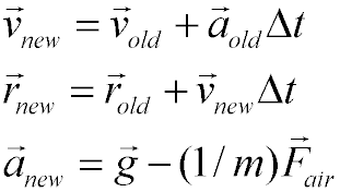
These are general equations that we will use next week when we encounter a variable acceleration (the effects of air resistance). For today's lab you can safely let a = g!
Your lab instructor will decide on whether you will do this either VPYTHON or EXCEL. Even though these are very different programs the underlying physics is the same!
- Prepare a simple flow chart that shows how these equations work together and also explain in your own words what each equation means.
- Next, using the values that you found in Part 1, set up a spreadsheet that uses these equations. Be sure to understand how to go from vector notation to component form in the spreadsheet!
- Set up a table in EXCEL that allows you to determine x and y coordinates (as well as vx and vy ) and prepare graphs of x-t, y-t and any others that you think would help demonstrate that your model works!
- You may use the file 2DTrajectory.xlsx to assist you but you will need to spend some time understanding how this file reproduces the equations given above.
What to Hand In
I would like the following from each lab group:
- neatly and appropriately labeled x-t and y-t tables and graphs with accompanying trendlines and equations clearly shown for Parts 1 and 3
- calculation showing how you found the initial velocity of the ball
- the value that your group found for "g" , a brief discussion of how you determined this and an estimate for the percentage error in this result.
- Discussion of how well your model worked and what factors influence its accuracy.
Date Due: One week from today