The Discovery of the Galaxy
Far out in the uncharted backwaters of the unfashionable end of the Western Spiral arm of the Galaxy lies a small unregarded yellow sun. Orbiting this at a distance of roughly ninety- eight million miles (sic) is an utterly insignificant blue- green planet whose ape-descendent life forms are so amazingly primitive that they still think digital watches are a pretty neat idea.
Where are We? |
|
Imagine you are blindfolded and taken to a shopping mall that you have never visited before. You are asked to sit at a small food court table and from there, once the blindfold is removed, draw as detailed a picture as you can of the entire complex - correct dimensions and all! Sound daunting? Perhaps to aid you you have a "special" telescope that allows you to see through walls (sorta) and even beyond the confines of the mall. This, is a rough analogy to what it is to be an astronomer fixed to the earth and yet trying to map out an entire galaxy. |
 |
| Figure 12.1 Sitting in an "average mall: anywhere in Canada - trying to understand what the mall looks like from the outside is analogous to our attempt to understand what our galaxy looks like. | |
Understanding the sun's relationship to other stars has been a remarkable intellectual journey. Coming to terms with the immense size of the universe is difficult even today. Historically the mapping of the universe beyond the solar system can be traced back to the time of Sir William Herschel (1738-1822), Caroline Herschel (1750 - 1848) and their contemporaries. Before we proceed it should be noted, however, that at the time of the Herschel's astronomy was dominated by the study of the solar system and comets. There was no clear sense of what a galaxy was let alone our own Milky Way.
Kant, Wright and Speculation
Several decades before he made his career by for ever more confusing philosophy students Immanuel Kant published (1755) a thin and surprisingly readable book called Cosmogony. In this book Kant attempts to demonstrate the mechanical nature of the universe and the ascendancy of Newton's Laws over "mystical" interventions. Kant also mused on the meaning of the Milky Way. Kant recognized that the Milky Way represented the disk-like structure of a vast swarm of stars - all orbiting some common center or centers in a manner very similar to the planets orbiting around the sun.Kant went on to speculate on the vastness of the universe:
The Infinitude of the creation is great enough to make a world, or a Milky Way of worlds, look in comparison with it what a flower or an insect does in comparison with the earth.At about the same time that Kant was musing about the Milky Way, the Englishman, Thomas Wright was publishing speculations on the nature of the Milky Way and the universe. Wright was a pious man and attempted, in his speculations, to determine the location of the Throne of God. His notion of God was a natural part of his many - unsuccessful - cosmogonies. But he did influence many people of his time (including Kant).
The Two Legs of Science: Herschel and His Telescopes
The popular view is that "Science advances on two legs: theory and observation". The advancement of our understanding of the Milky Way had to await the observational genius of Herschel.
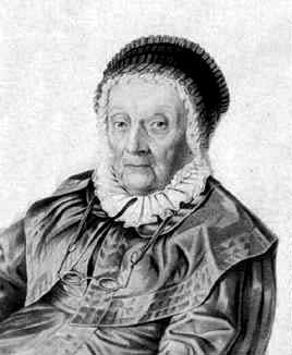
Sir William Herschel (Figure 12.2) was, by training, an oboist-composer and not a scientist at all . Born in Germany, he emigrated to Britain in 1757. By 1766 he was organist at the Octagon Chapel at Bath. It was during this time that his interest in optics and astronomy was kindled. By 1773 he had made his first telescope. Eventually he became so proficient that his telescopes far outstripped the telescopes in use by the "professional" astronomers of his day. In 1776 Herschel completed the "20 foot" telescope. His telescopes now far exceeded in both size and quality the instruments of his professional contemporaries. With these powerful new telescopes Herschel began to peer into the heavens and discover a wealth and complexity unknown before that time. Herschel was a "naturalist" of the heavens and, with the indispensable aid of his sister Caroline (Figure 12.3), began to painstakingly record and draw the things which he saw. In 1781 Herschel made a significant discovery. He discovered the planet Uranus which he wisely named Georgium Sidus (Georgian star) and promptly collected a lifetime pension from King George III! No more music for Herschel, he retired comfortably to a new abode near Windsor Castle. His only duty was to be "on call" as the court astronomer. He was rich and famous and devoted the rest of his life to charting the sky. What the Herschel's found was a rich feast of diverse objects from nebulous patches to clusters of stars. Herschel's work extended greatly the cataloguing work done by his French contemporary Charles Messier. What Herschel also began to show was the vastness of the sky. Perhaps some of these nebulous "blobs" were themselves separate "Milky Ways". The "modern" view of the universe was incipient in the observations of the Herschel's In honor of the Herschel's importance to both astronomy and telescope technology the William Herschel Telescope has been commissioned. It i part of the Isaac Newton Group of telescopes described in Chapter 5.2. |
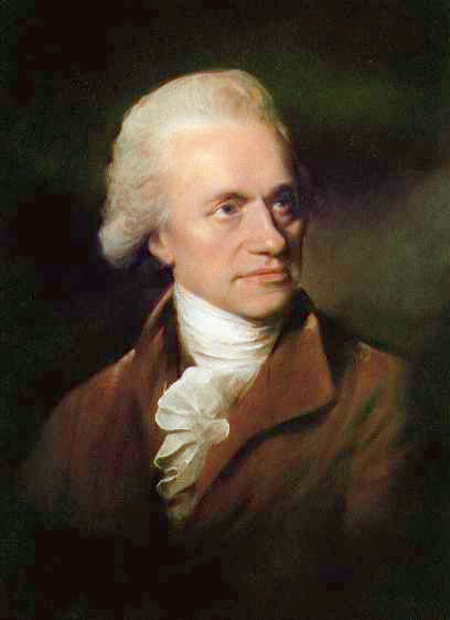 |
| Figure 12.2 Sir William Herschel (1738-1822) (image in public domain) | |
 |
|
| Figure 12.3 Caroline Herschel (1750-1848) (image in public domain) |
The Grindstone Model and Others
Through painstaking star counts made in different directions Herschel envisioned the Milky Way as a flat "grindstone" of stars with the sun situated roughly at the center. Using the common grindstone as a model, Herschel conjectured that the dark lanes seen in the Milky Way for example, implied that the edge of the "grindstone" was irregular. The roll-over image in Figure 12.4 illustrates this. The size of the galaxy was still on a matter of conjecture. By about 1900 a crude idea of the size of the galaxy was available but still there was no notion of the galaxy in relation to the vastness of the universe. A particular source of speculation was the nature of the "nebulae" and the "island universe" idea. |
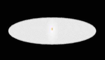 |
| Figure 12.4 The grindstone model of the galaxy. |
Herschel's telescopes were odd and ungainly objects. To see the last great telescope of this design (The Lord Rosse telescope in Birr, Ireland) follow the "Take a Closer Look" link.

While Herschel had only a vague notion of the shape of the Milky Way galaxy he had even less understanding of its size. This knowledge had to wait until the beginning of the 20th century with the work of Henrietta Leavitt and her study of variable stars.
Stellar Variability and the Period-Luminosity Relation
But I am as constant as the northern
star,
Of whose true-fix'd and resting quality
There is no fellow in the firmament
Keen observers of the night sky have known, probably for millennia, that some stars are not "constant". Indeed, the North Star itself varies in brightness. More than mere curiosities, however, variable stars provide astronomers with a valuable "standard candle" to plumb the vast distances of space.
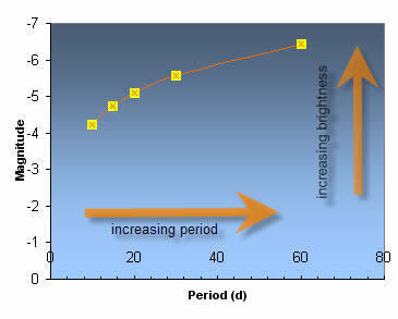
The first successful use of variables stars as distance indicators came from the work of American astronomer Henrietta Leavitt. In 1912 Leavitt announced an intriguing find. She had been studying Cepheid Variable stars in the nearby Magellanic Clouds. Cepheids are very bright stars with light variation typically on the order of a magnitude or less and with periods of a few days to several months. The Magellanic clouds are close by "satellite galaxies" visible from the southern hemisphere. Leavitt discovered that the longer the period of variation the brighter the star. This relationship can be given a precise mathematical form and is called the Period-Luminosity Relation.
| Figure 12.5 |
Example 12.1 Use the applet VariableStar to investigate the relationship between the period of a Cepheid variable (Tpye I) and its absolute visual magnitude.
Solution: To use the applet, select the period that you would like and then press "plot" (lower right corner). Let the star oscillate through a number of cycles before you press the pause button. Note the Average Absolute Visual Magnitude MV which is shown on the left with other information about the star. The following table and graph show typical data you might expect to collect.
|
 |
|||||||||||||
| Representative data and resulting P-L graph for Type I Cepheids | ||||||||||||||
You can also see the period-magnitude data plotted if you select the "Period-Magnitude" tab on the bottom graph in the applet.
As example 12.1 shows, Cepheid variable stars are very bright and thus can be seen at great distances. The period-luminosity relationship also means that by measuring the period (a relatively easy thing to do) you get the absolute magnitude as a "bonus". Knowing this and the apparent magnitude you can determine the distance modulus use the techniques developed in Chapter 8.2 to determine the distance of the star.
Example 12.2 A Type I Cepheid is discovered in a remote part of the galaxy. Careful observation over several months reveals that the star has an average apparent magnitude of 6.81 and a period of 28.5 days. Estimate the distance to this star.
Solution: Use ![]() VariableStar to help answer this. The Period-Luminosity relationship implies that the absolute visual magnitude should be -5.52. This means that the distance modulus for this star is mV - Mv = 6.81 - (-5.52) = 12.33. If you use the
VariableStar to help answer this. The Period-Luminosity relationship implies that the absolute visual magnitude should be -5.52. This means that the distance modulus for this star is mV - Mv = 6.81 - (-5.52) = 12.33. If you use the ![]() distanceModulus to determine the distance. If you do this you will discover that the star is 2930 pc (2.93 kpc) away.
distanceModulus to determine the distance. If you do this you will discover that the star is 2930 pc (2.93 kpc) away.
Henrietta Leavitt's discovery of the period-luminosity relation gave astronomers the tool that they needed to begin an exploration of the galaxy. By the early 1920's it was clear that distances in the galaxy must be measured in 10's of thousands of light years.
Stellar Pulsation - A Closer Look
What causes a Cepheid Variable to change in brightness? In the previous unit we encountered binary star systems in which variation in brightness could be due to eclipses, distortion in the shapes of the stars or both. Cepheid Variables, on the other hand, belong to a group of stars called intrinsic variables - they vary in brightness because they also vary in size and temperature. The reason for this variation is complex (follow the "Take a Closer Look" link below to learn more). Essentially stellar pulsation occurs because in some stars a layer of partially ionized helium can act as a "valve" or spring that can absorb and release energy. If the temperature and density of the layer in which this occurs is "just right" then this will lead to a rhythmic expansion and contraction of the star which also leads to variation in brightness. It turns out that most stars will at some point in their evolution become, for a short period of time, pulsating variables. This can be shown on the Hertzsprung-Russel Diagram. Figure 12.6 illustrates this using the applet starEvelove. There are several distinct regions on the HR-diagram called Instability Strips in which a star can undergo pulsation.
| Figure 12.6 |
Example 12.3 Use the applet starEvolve to compare the time that a 5 Mo star will spend in the instability strip with the time that a 2.5 Mo star will spend in the instability strip.
Solution: Double click the radio buttons for the 5 Mo and 2.5 Mo and then use the slider to step through the evolutionary models for each star. The info panel on the lower left will show you the age of the star since it joined the Zero-Age Mains Sequence (ZAMS). Because more massive stars evolve much faster you can see that a5 Mo star spends less than 100 thousand years in the instability strip while a 2.5 Mostar spends about 85 million years in the instability strip.
Other Kinds of Intrinsic Variable Stars
|
Figure 12.6 shows a number of star types and two instability strips. This is because there are a number of different classes and sub-classes of intrinsic variables. The main ones are summarized in Table 12.1. Figure 12.7 shows the light curve for the star DY-Pegasi which is a member of a sub-class of the Cepheids stars called the SX-Phoenicis stars. This is similar to a Cepheid but with a period of an hour or so! In most cases the variable class is named after the first star of its type to be discovered. | |||||||||||||||||||||||||||||||||||||||||||||
Figure 12.7 DY-Pegasi ( a member of the SX-Phoenicis sub-class) |
The Problem of Calibration and The Size of the Milky Way
Leavitt's discovery of the Period-Luminosity had a "snag". In order to use it to determine distances you would first need to know the absolute magnitudes of the variables that you were studying. Leavitt did not have this critical piece of information needed to calibrate the P-L relation. This problem was solved by the American astronomer Harlow Shapley who was able to determine the absolute magnitude of a small number of relatively nearby Cepheids. Once having calibrated the P-L relationship Shapley had a powerful tool at his disposal and this led quickly to an understanding of both the approximate size of the galaxy as well as our place in the galaxy.
To determine the size of the galaxy and our location in it Shapley studied the distribution of globular clusters in the sky. You first encountered globular clusters in Chapter 10.1. Figure 12.8 shows an example of a globular cluster - M55 which is found in the constellation Sagittarius. M55 is one of about 150 known globular clusters associated with our galaxy. Shapley was able to locate RR-Lyrae variables in these clusters and from this determine their distance from us. When this was plotted along with their position in the sky a very revealing insight emerged. Figure 12.9 gives you an applet that allows you to inspect more modern data on the known globular clusters. The data is taken from the work of William Harris of McMaster University. When you interact with the data see if you can visualize what this is telling you about the size of the galaxy and where we are in it. |
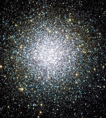 |
Figure 12.8 Globular cluster M55 in Sagittarius. (Image courtesy Canada-France-Hawaii Telescope / Coelum) |
| Figure 12.9 |
Example 12.4 In 1900 astronomers thought that the Milky Way was likely a disk-like shape with the Sun situated at the center of the Milky Way. Does the distribution provided in ![]() globularCluster support this conclusion?
globularCluster support this conclusion?
Solution: The disk-like shape of the galaxy was known to Herschel and derives from the simple observation that the density of stars is highest in a band of the sky (the Milky Way). However, the data shown in Figure 12.9 does not support the claim that the Sun is at the centre of the Milky Way. THe reason is that the globular clusters are clearly spherically distributed about another point than the Sun (shown in yellow). Shapley made the correct assumption that the globular clusters would orbit around the centre of the galaxy.
Shapley's study of the distribution of globular clusters revealed that the Sun is situated many thousands of light years away from the centre of the Milky Way galaxy. Shapley was one of the first astronomers to understand the true size of the galaxy.
The Shapley-Curtis Debate
By 1920 astronomers began to realize that not only was the Milky Way big but that perhaps there were other "Milky Ways". What we now know as external galaxies were, up to that time, a mystery. Some, Shapley included, thought they were parts of our own Milky Way while others, notably Heber Curtis suggested that they were independent bodies like our own Milky Way. They used the term "Island Universes" to describe them. This marked disagreement led, eventually to an important debate in early 20th century astronomy.
More often than not scientific debates create more heat than light and at times can even generate a "side-show" atmosphere. This is true of a disagreement between Shapley and Heber Curtis which centered around two points:
- the size of the galaxy
- the nature of the nebulae
Shapley: |
|
|
Curtis: |
|
| Table 12.2 Summary of the Shapley-Curtis points of debate |
Curtis favoured the "island universe" idea which held that some of the nebulae observed were actually independent galaxies and the galaxy was actually much smaller than Shapley suggested. This debate attracted a lot of attention in the early 1920's and was really a series of arguments and counter-arguments carried out by Shapley and Curtis in the "press" (scientific journals) as well as at conferences.
In the end it turned out that both men were right (and wrong!) - these ideas need not exclude each other. If you wish you may follow this link to view a transcript of the debate.
 To understand the structure and size of our galaxy
Chp 15.1
322-326
![]()
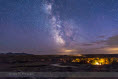
The Milkyway from Writing on Stone Provincial Park in Southern Alberta. Check out Alan Dyer's site!
258-262
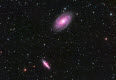
Nearby galaxies M81 and M82