Quasars
380-386
In the early 1960's two very blue, star-like objects were observed in the same region of the sky from which strong radio emissions were also detected. This spawned a whole flurry of theories about radio stars. These theories turned out to be fictions and the truth much stranger! Quasars are not only enigmatic - they have also become extremely important tools for probing the farthest reaches of the cosmos.
Quasars and Red shifts
In 1962 the astronomer Maarten Schmidt astonished the astronomical community by showing that the red shifts of the "quasi-stellar" objects were enormous - much larger than any previously known red shifts for galaxies. One of the objects - 3C 273 had a redshift 0f 0.15 while another, 3C 48 has a red shift of 0.37! This was part of the problem in identifying the spectra of these objects. The spectral lines were red shifted by such an enormous amount that lines normally visible only in the ultraviolet were shifted into the visible region. Once this was realized it was realized that astronomers were looking at very unusual objects. Figure 14.8 shows quasar 3C 273 and a peculiar jet emanating from the object. Figure 14.9 shows the Hydrogen Balmer-line spectrum for this object. The red, vertical line represents the position you would expect to see the Balmer-alpha line at. Instead, the line is shifted far to the right indicating a very large redshift. The other Balmer lines are also shown redshifted far from their "laboratory" positions.
 |
 |
| Figure 14.8 Image of quasar 3C 273 | Figure 14.9 Spectrum of 3C 273 |
Redshifts are denoted by the letter "z" and defined by the formula:
In this equation ![]() is the wavelength of the shifted line while
is the wavelength of the shifted line while ![]() is the wavelength that you would measure in the lab (the "rest frame wavelength").
is the wavelength that you would measure in the lab (the "rest frame wavelength").
Example 14.4 The Hydrogen Balmer-alpha line in 3C 273 is measured at a wavelength of 760 nm rather than its rest frame wavelength of 656 nm. What is the z-value (redshift) for this line?
Solution: Set this up using the redshift formula:
Redshifts and Apparent Recessional Velocity
At low velocity (less than about 15% the speed of light) the z-value of a redshifted object is almost equal to the recessional velocity of the object expressed as a fraction of the speed of light. This means that if z = 0.10 then the object producing this light has a recessional velocity of v/c = 0.1 or v = 0.1c.
Example 14.5 How fast is 3C 273 receding from Earth? Express the answer in both "light units" and km/s.
Solution: Since z = 0.158 we can interpret this to mean that 3C 273 is moving away from us at nearly 15.8% the speed of light. In "light units" this is v/c = 0.158 or v = 0.158c. To convert this to km/s just replace c by 300 000 km/s. This gives v = (0.158)(300 000 km/s) = 47,400 km/s!
For redshifts larger than 0.15 there is a more sophisticated equation that accounts for effects predicted by Einstein's Special Theory of Relativity. When this is applied to the case of 3C 273 the velocity is 0.146 rather than 0.158.

Figure 14.10 provides the applet quasar that you can use to show how recessional velocity will shift a star or galaxy's spectrum. You can also use the "Z-Calculator" to determine z-values and recessional velocity.
| Figure 14.10 |
Example 14.6 The hydrogen Balmer line He is measured to be 810 nm (in the infrared!) for a distant quasar. What z value does this imply? Use the calculator part of the applet quasar to determine the recessional velocity.
Solution: The applet indicates that z = 1.04 in this case and this corresponds to a recessional velocity of 0.612 c or about 180 000 km/s.
What Redshift Recessional Velocities are NOT
A popular misconception is that if you were near a quasar such 3C 237 or 3C 48 it would "whiz by" at an enormous velocity. It would not! When we talk about recessional velocity we are really talking about the rate of expansion of the universe itself. You would not see the quasar whiz past because you would share in the same expansion of the universe and would move along with the quasar. To a distant observer both you and the quasar would appear to be receding at high velocity. When we apply the Doppler formula for velocity it is important to realize that for distant galaxies the apparent recessional velocity is really a combination of two effects: the intrinsic motion of the galaxy itself relative to you and the expansion of the universe. We will explore the idea of the expanding universe in more detail in the next unit.
Quasars, Distance and Brightness
What was so startling about the discovery of quasars in the early 1960's was their distance and implied intrinsic brightness. To understand this consider the next two examples.
Example 14.7 Use the Hubble Expansion Law from Chapter 13.2 to determine the distance to quasar 3C 273.
Solution: Recall that the Hubble Expansion Law connects recessional velocity to distance by the simple formula:
 . In the formula H is Hubble's constant and has the value 71 km/s/Mpc. In Example 14.5 you determined that v = 47,400 km/s so...
This gives r = 668 Mpc or over 2 billion light years! (you can also use the Applet ![]() Hubble Expansion to do this!)
Hubble Expansion to do this!)
In Example 14.6 you are making the Cosmological Assumption. This means that you interpreted the redshift and accompanying velocity as a measure of expansion of the universe. This is what the Hubble Expansion Law is measuring.
Example 14.8 Quasar 3C 273 has an apparent magnitude of 13. What intrinsic brightness (absolute magnitude) does this imply for 3C 273?
Solution: This is just a distance modulus problem! So - you can either use the applet ![]() dMOd or the distance modulus formula m-M = 5log(d/10) to answer this. We will use the applet and get the result that m-M = 39! This tells us that the absolute magnitude M = -26. The absolute magnitude of our galaxy is -20.5 so this implies that 3C 273 is much brighter than a normal galaxy. In the case of 3C 273 it is about 300 times brighter than our galaxy.
dMOd or the distance modulus formula m-M = 5log(d/10) to answer this. We will use the applet and get the result that m-M = 39! This tells us that the absolute magnitude M = -26. The absolute magnitude of our galaxy is -20.5 so this implies that 3C 273 is much brighter than a normal galaxy. In the case of 3C 273 it is about 300 times brighter than our galaxy.
Quasar Variability and Similarity with AGN's
It was soon discovered that quasars are variable in luminosity. Time scales for variation can be a short as a few hours which implies that what ever is producing the enormous energy of the quasar is confined to a tiny region about the size of our solar system. Does this sound familiar? As well, there is a curious difference between the redshifts of emission lines compared to absorption lines in quasars. Figure 14.11 shows this.
 |
In this image the redshifts for roughly 2000 quasars are plotted. The clustering of data points in the lower corner of the graph means that the redshift for any given quasar will be higher for emission lines than absorption lines. This is a clue that tells us something about what a quasar really is. The emission lines observed are most likely produced in a tiny region in the quasar itself. The absorption lines are likely due to absorption by the intervening material between the quasar and Earth-based observers. We will return to this in the next unit and use this to argue that quasars really are extremely distant objects. |
| Figure 14.11 Plot that shows that emissions lines systematically show higher z-values than absorption lines. These are data from a sample of 2000 quasars. |
A Model for Quasars
It should come as no surprise that our model for quasars is essentially the same one that we created for AGN's. Figure 14.8 shows a jet structure on 3C 273 that is very much like the jets and radio lobes seen on AGN's. Many quasars are also radio-lobed galaxies and all of this points to a similar conclusion - quasars are powered by accretion around supermassive black holes.
Quasars and the History of the Universe
Figure 14.11 shows a few quasar redshifts above z = 4 but most are concentrated around 2. What does this mean? If you determine the distance implied by z = 2 you would find that the "typical" distance for quasars is about 10 billion light years. Another way to think about this, however, is to recall the concept of look-back time. The clustering of quasar redshifts is telling something about the universe 10 billion years ago! At that time the quasars were forming and actively colliding. In this "age of quasars" they were about 1000 times more common than they are today.
Example 14.9 Figure 14.12 shows a composite image of the Canada-France-Hawaii telescope and the discovery image and spectrum of the most distant quasar known - CFHQS J2329-0301. In the spectrum inset, the hydrogen Lyman-alpha line, normally at l = 121.6 nm (far in the ultraviolet) is shifted to 904 nm (in the infrared)! Estimate the "age" or look-back time for when this quasar formed.
Solution: Use the calculator in applet quasar to help answer this as well as the Hubble Expansion Law. From the applet you find:
Convert the velocity (0.964c) to km/s to get v = 289 000 km/s and apply
From this you find that r = 4.07 billion parsecs = 13.3 billion light years. This quasar formed about 13 billion years ago - very early in the history of the universe.
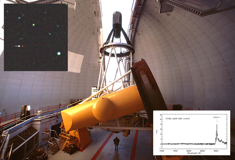 |
| Figure 14.12 Composite image of the Canada-France-Hawaii telescope and the most distant known quasar CFHQS J2329-0301 along with its identification spectrum. |
Practice
- When quasars were first discovered some astronomers suggested that they were small masses ejected from the nuclei of galaxies. What piece of observational evidence argues against this hypothesis?
- If the Balmer Hb line is observed to occur with a wavelength of 600 nm what redhsift z-value should you record for this quasar?
- Shown below is a low resolution spectrum of the Quasar 3C273 taken at The King's University Observatory


April 2011. The positions of the Hydrogen alpha (red) and Hydrogen beta (blue -green) are shifted to wavelengths 760 nm and 562 nm resepectively. From this determine the recessional velocity of this quasar and estimate its distance. - The apparent magnitude of 3C 273 is 12.9. Using what you calculated in question 3 estimate the absolute magnitude of this galaxy.
- What evidence is there that supports the idea that quasars are triggered through galactic collision and merger?
- Discuss - is it possible that our own galaxy was a quasar at one time?

To understand what Quasars are and how they are used to "measure" the cosmos
Chp 17.2
 Since their discovery the name for quasars has undergone its own evolution from "Quasi-stellar
object" and "Quasi-stellar Radio Sources" to finally just "Quasars".
Since their discovery the name for quasars has undergone its own evolution from "Quasi-stellar
object" and "Quasi-stellar Radio Sources" to finally just "Quasars".
The redshift of 3C273 was measured in a recent King's student's 4th year thesis

The Doppler Effect
